13. SymPy#
Contents
13.1. Overview#
Unlike numerical libraries that deal with values, SymPy focuses on manipulating mathematical symbols and expressions directly.
SymPy provides a wide range of features including
Symbolic Expression
Equation Solving
Simplification
Calculus
Matrices
Discrete Math, etc.
These functions make SymPy a popular open-source alternative to other proprietary symbolic computation software such as Mathematica.
In this lecture, we will explore some of the functionalities of SymPy and demonstrate how to use basic SymPy functions to solve economic models.
13.2. Getting Started#
Let’s first import the library and initialize the printer for symbolic output
from sympy import *
from sympy.plotting import plot, plot3d_parametric_line, plot3d
from sympy.solvers.inequalities import reduce_rational_inequalities
from sympy.stats import Poisson, Exponential, Binomial, density, moment, E, cdf

import numpy as np
import matplotlib.pyplot as plt

# Enable the mathjax printer
init_printing(use_latex='mathjax')
13.3. Symbolic algebra#
13.3.1. Symbols#
Before we start manipulating the symbols, we initialize some symbols to work with
x, y, z = symbols('x y z')
Symbols are the basic units for symbolic computation in SymPy.
13.3.2. Expressions#
We can now use symbols x, y, and z to build expressions and equations.
Here we build a simple expression first
expr = (x+y) ** 2
expr
We can expand this expression with the expand function
expand_expr = expand(expr)
expand_expr
and factorize it back to the factored form with the factor function
factor(expand_expr)
We can solve this expression
solve(expr)
Note this is equivalent to solving the following equation for x
Another way to solve this equation is to use solveset.
solveset allows users to define the domain of x in the evaluation and output a set as a solution
solveset(expr, x, domain=S.Naturals)
Note
Solvers is an important module with tools to solve different types of equations.
There are a variety of solvers available in SymPy depending on the nature of the problem.
13.3.3. Equations#
SymPy provides several functions to manipulate equations.
Let’s develop an equation with the expression we defined before
eq = Eq(expr, 0)
eq
Solving this equation with respect to \(x\) gives the same output as solving the expression directly
solve(eq, x)
SymPy can handle equations with multiple solutions
eq = Eq(expr, 1)
solve(eq, x)
solve function can also combine multiple equations together and solve a system of equations
eq2 = Eq(x, y)
eq2
solve([eq, eq2], [x, y])
We can also solve for the value of \(y\) by simply substituting \(x\) with \(y\)
expr_sub = expr.subs(x, y)
expr_sub
solve(Eq(expr_sub, 1))
Below is another example equation with the symbol x and functions sin, cos, and tan using the Eq function
# Create an equation
eq = Eq(cos(x) / (tan(x)/sin(x)), 0)
eq
Now we simplify this equation using the simplify function
# Simplify an expression
simplified_expr = simplify(eq)
simplified_expr
Again, we use the solve function to solve this equation
# Solve the equation
sol = solve(eq, x)
sol
SymPy can also handle more complex equations involving trigonometry and complex numbers.
We demonstrate this using Euler’s formula
# 'I' represents the imaginary number i
euler = cos(x) + I*sin(x)
euler
simplify(euler)
If you are interested, we encourage you to read the lecture on trigonometry and complex numbers.
13.3.3.1. Example: fixed point computation#
Fixed point computation is frequently used in economics and finance.
Here we solve the fixed point of the Solow-Swan growth dynamics:
where \(k_t\) is the capital stock, \(f\) is a production function, \(\delta\) is a rate of depreciation.
With \(f(k) = Ak^a\), we can show the unique fixed point of the dynamics using pen and paper:
This can be easily computed in SymPy
A, s, k, α, δ = symbols('A s k_t α δ')
# Define Solow-Swan growth dynamics
solow = Eq(s*A*k**α + (1-δ)*k, k)
solow
solve(solow, k)
13.3.4. Inequalities and logic#
SymPy also allows users to define inequalities and set operators and provides a wide range of operations.
reduce_inequalities([2*x + 5*y <= 30, 4*x + 2*y <= 20], [x])
And(2*x + 5*y <= 30, x > 0)
13.3.5. Series#
Series are widely used in economics and statistics, from asset pricing to the expectation of discrete random variables.
We can construct a simple series of summations using Sum function and Indexed symbols
x, y, i, j = symbols("x y i j")
sum_xy = Sum(Indexed('x', i)*Indexed('y', j),
            (i, 0, 3),
            (j, 0, 3))
sum_xy
To evaluate the sum, we can lambdify the formula.
The lambdified expression can take numeric values as input for \(x\) and \(y\) and compute the result
sum_xy = lambdify([x, y], sum_xy)
grid = np.arange(0, 4, 1)
sum_xy(grid, grid)
36
13.3.5.1. Example: bank deposits#
Imagine a bank with \(D_0\) as the deposit at time \(t\).
It loans \((1-r)\) of its deposits and keeps a fraction \(r\) as cash reserves.
Its deposits over an infinite time horizon can be written as
Let’s compute the deposits at time \(t\)
D = symbols('D_0')
r = Symbol('r', positive=True)
Dt = Sum('(1 - r)^i * D_0', (i, 0, oo))
Dt
We can call doit method to evaluate the series
Dt.doit()
Simplifying the expression above gives
simplify(Dt.doit())
This is consistent with the solution in the lecture on geometric series.
13.3.5.2. Example: discrete random variable#
In the following example, we compute the expectation of a discrete random variable.
Let’s define a discrete random variable \(X\) following a Poisson distribution:
λ = symbols('lambda')

# We refine the symbol x to positive integers
x = Symbol('x', integer=True, positive=True)
pmf = λ**x * exp(-λ) / factorial(x)
pmf
We can verify if the distribution follows the fundamental property of probability distribution:
sum_pmf = Sum(pmf, (x, 0, oo))
sum_pmf.doit()
The expectation of the distribution is:
fx = Sum(x*pmf, (x, 0, oo))
fx.doit()
SymPy includes a statistics module called Stats.
Stats module offers built-in distributions and functions on probability distributions.
The computation above can also be condensed into one line using the expectation function E in the Stats module
λ = Symbol("λ", positive = True)

# Using sympy.stats.Poisson() method
X = Poisson("x", λ)
E(X)
13.4. Symbolic Calculus#
SymPy allows us to perform various calculus operations, such as limits, differentiation, and integration.
13.4.1. Limits#
We can compute limits for a given expression using the limit function
# Define an expression
f = x**2 / (x-1)

# Compute the limit
lim = limit(f, x, 0)
lim
13.4.2. Derivatives#
We can differentiate any SymPy expression using the diff function
# Differentiate a function with respect to x
df = diff(f, x)
df
13.4.3. Integrals#
We can compute definite and indefinite integrals using the integrate function
# Calculate the indefinite integral
indef_int = integrate(df, x)
indef_int
Let’s use this function to compute the moment-generating function of exponential distribution with the probability density function:
λ = Symbol('lambda', positive=True)
x = Symbol('x', positive=True)
pdf = λ * exp(-λ*x)
pdf
t = Symbol('t', positive=True)
moment_t = integrate(exp(t*x) * pdf, (x, 0, oo))
simplify(moment_t)
Note that we can also use Stats module to compute the moment
X = Exponential(x, λ)
moment(X, 1)
E(X**t)
Using the integrate function, we can derive the cumulative density function of the exponential distribution with \(\lambda = 0.5\)
λ_pdf = pdf.subs(λ, 1/2)
λ_pdf
integrate(λ_pdf, (x, 0, 4))
Using cdf in Stats module gives the same solution
cdf(X, 1/2)
# Plug in a value for z
λ_cdf = cdf(X, 1/2)(4)
λ_cdf
# Substitute λ
λ_cdf.subs({λ: 1/2})
13.5. Plotting#
SymPy provides a powerful plotting feature.
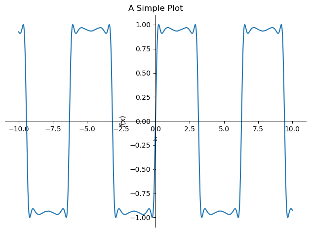
First we plot a simple function using the plot function
f = sin(2 * sin(2 * sin(2 * sin(x))))
p = plot(f, (x, -10, 10), show=False)
p.title = 'A Simple Plot'
p.show()
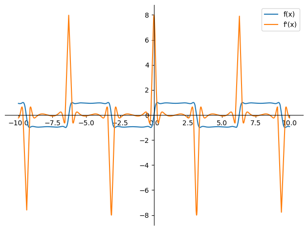
Similar to Matplotlib, SymPy provides an interface to customize the graph
plot_f = plot(f, (x, -10, 10),
              xlabel='', ylabel='',
              legend = True, show = False)
plot_f[0].label = 'f(x)'
df = diff(f)
plot_df = plot(df, (x, -10, 10),
            legend = True, show = False)
plot_df[0].label = 'f\'(x)'
plot_f.append(plot_df[0])
plot_f.show()
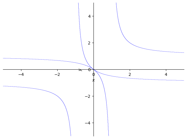
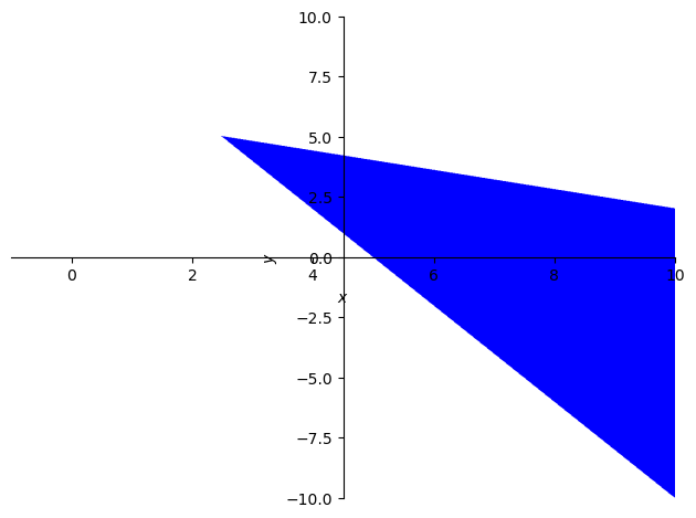
It also supports plotting implicit functions and visualizing inequalities
p = plot_implicit(Eq((1/x + 1/y)**2, 1))
p = plot_implicit(And(2*x + 5*y <= 30, 4*x + 2*y >= 20),
                     (x, -1, 10), (y, -10, 10))
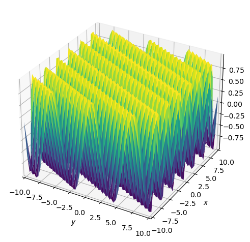
and visualizations in three-dimensional space
p = plot3d(cos(2*x + y), zlabel='')
13.6. Application: Equalizing Differences Model#
In this section, we apply SymPy to construct an equalizing differences model that explores the choice between going to college and working directly after high school.
In this example, imagine a student deciding whether to be admitted into a college or entering the workforce after high school.
The student is indifferent between the two options if the present values of the earnings from the two options are the same.
For more details on the model, please visit the lecture on equalizing differences model.
13.6.1. Defining the Symbols#
The first step in symbolic computation is to define the symbols that represent the variables.
In our model, we need the following variables:
\(R > 1\) be the gross rate of return on a one-period bond
\(t = 0, 1, 2, \ldots T\) denote the years that a person either works or attends college
\(0\) denotes the first period after high school that a person can go to work
\(T\) denotes the last period that a person works
\(w_t^h\) be the wage at time \(t\) of a high school graduate
\(w_t^c\) be the wage at time \(t\) of a college graduate
\(\gamma_h > 1\) be the (gross) rate of growth of wages of a high school graduate, so that wage for high school graduates at time \(t\) is \( w_t^h = w_0^h \gamma_h^t\)
\(\gamma_c > 1\) be the (gross) rate of growth of wages of a college graduate, so that wage for college graduates at time \(t\) is \( w_t^c = w_0^c \gamma_c^t\)
Let’s define these symbols using SymPy
# Define the symbols
R, wh0, wc0, γ_c, γ_h, t, T = symbols(
    'R w^h_0 w^c_0 gamma_c gamma_h t T', positive=True)

refine(γ_c, γ_c>1)
refine(γ_h, γ_h>1)
refine(R, R>1)

# Define the wage for college
# and high school graduates at time t
w_ct = wc0 * γ_c**t
w_ht = wh0 * γ_h**t
w_ct
w_ht
13.6.2. Defining the Present Value Equations#
The present value of the earnings after going to college is
It is the sum of the discounted earnings from the first year of graduation to the last year of work assuming the degree is obtained in the fourth year and no salary is earned while in the college.
The present value of the earnings from going to work after high school is
It is the sum of the discounted earnings from the first year after high school to the last year of work.
PV_college = Sum(R**-t * w_ct, (t, 4, T))
PV_college
PV_highschool = Sum(R**-t * w_ht, (t, 0, T))
PV_highschool
We can evaluate the sum using the doit method
PV_hs = simplify(PV_highschool.doit())
PV_hs
PV_c = simplify(PV_college.doit())
PV_c
13.6.3. Defining the Indifference Equation#
Now we introduce the symbol \(\phi\) to represent the fraction of high school graduates who go to college and \(D\) to represent the upfront monetary costs of going to college.
D, ϕ = symbols('D phi', positive=True)
We can solve for by solving the equation below with regards to \(\phi\)
so that
When \(\phi\) is greater than 1, the person will choose to go to work.
When \(\phi\) is less than 1, the person will choose to go to college.
When \(\phi\) is equal to 1, the person is indifferent between going to college and going to work.
Let’s solve for \(\phi\) using SymPy
indifference = Eq(PV_hs.args[1][0],
                  ϕ*PV_c.args[1][0] - D)
indiff_sol = solve(indifference, ϕ)[0]
indiff_sol
Using Lambda function, we can specify the parameters of the equation
lambda_indiff = Lambda((R, wh0, wc0, γ_c, γ_h, D, T),
                indiff_sol)
lambda_indiff
We use the following parameters to compute the value for \(\phi\)
R_value = 1.05
γ_c_value, γ_h_value = 1.01, 1.01
wh0_value = 1
wc0_value = 2
D_value = 10
T_value = 40

lambda_indiff(R_value, wh0_value, wc0_value,
              γ_c_value, γ_h_value, D_value,
              T_value)
Under this setting, we find college is more attractive to the person as \(\phi < 1\).
Note that we can also use the subs method to substitute the values of the parameters
indiff_sol.subs({R: R_value,
                wh0: wh0_value,
                wc0: wc0_value,
                γ_c: γ_c_value,
                γ_h: γ_h_value,
                D: D_value,
                T: T_value})
It is also possible to use the evalf method to get floating-point approximations
indiff_sol.evalf(subs={R: R_value,
                      wh0: wh0_value,
                      wc0: wc0_value,
                      γ_c: γ_c_value,
                      γ_h: γ_h_value,
                      D: D_value,
                      T: T_value})
Note how precision changes using different methods.
We encourage readers to read more about how SymPy uses different methods to evaluate a function/expression.
As a recap, we can lambdify a function to take a range of values.
For instance, we want to know how \(\phi\) changes with different time lengths \(T\) (expected years of work)
indiff_sol_T = indiff_sol.subs({R: R_value,
                                wh0: wh0_value,
                                wc0: wc0_value,
                                γ_c: γ_c_value,
                                γ_h: γ_h_value,
                                D: D_value})
plt.plot(np.arange(10, 60, 1),
         lambdify(T, indiff_sol_T)(np.arange(10, 60, 1)))
plt.xlabel('T')
plt.ylabel(r'$\phi$')
plt.show()
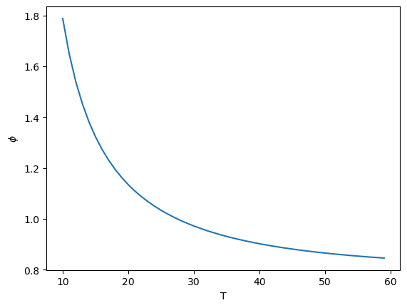
As \(T\) increases, \(\phi\) decreases favoring attending college.
indiff_sol_TD = indiff_sol.subs({R: R_value,
                                wh0: wh0_value,
                                wc0: wc0_value,
                                γ_c: γ_c_value,
                                γ_h: γ_h_value})
What if we want to know how \(\phi\) changes with different tuition fees \(D\) and \(T\)?
grid = np.meshgrid(np.arange(10, 60, 1),
                   np.arange(0, 60, 1))
ϕ_TR = lambdify([T, D], indiff_sol_TD)(grid[0], grid[1])
fig = plt.figure()
ax = plt.axes(projection ='3d')
ax.set_box_aspect(aspect=None, zoom=0.85)

ax.plot_surface(grid[0],
                grid[1],
                ϕ_TR)
ax.set_xlabel('T')
ax.set_ylabel('D')
ax.set_zlabel(r'$\phi$')
plt.show()
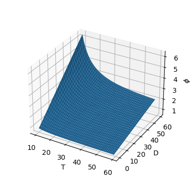
We can see how \(\phi\) flats out when we increase the time horizon as college graduates have higher salary at different levels of tuition fee.
A student facing a shorter expected working period and higher tuition fee prefers to work directly after high school.
Let’s take a step further by taking the derivative of \(\phi\) with respect to \(D\) to compute the marginal effect of tuition fee on \(\phi\)
diff_D = lambda_indiff(R, wh0, wc0,
                       γ_c, γ_h, D, T).diff(D)
simplify(diff_D)
diff_D_func = Lambda((R, wh0, wc0,
                      γ_c, γ_h, D, T), diff_D)
We can see that higher tuition fee gives more incentives for high school graduates to go to work directly.
diff_D_func(R_value, wh0_value, wc0_value,
            γ_c_value, γ_h_value, D_value,
            T_value)
13.7. Exercises#
Exercise 13.1
L’Hôpital’s rule states that for two functions \(f(x)\) and \(g(x)\), if \(\lim_{x \to a} f(x) = \lim_{x \to a} g(x) = 0\) or \(\pm \infty\), then
Use SymPy to verify L’Hôpital’s rule for the following functions
as \(x\) approaches to \(0\)
Solution to Exercise 13.1
Let’s define the function first
f_upper = y**x - 1
f_lower = x
f = f_upper/f_lower
f
Sympy is smart enough to solve this limit
lim = limit(f, x, 0)
lim
We compare the result suggested by L’Hôpital’s rule
lim = limit(diff(f_upper, x)/
            diff(f_lower, x), x, 0)
lim
Exercise 13.2
Maximum likelihood estimation (MLE) is a method to estimate the parameters of a statistical model.
It usually involves maximizing a log-likelihood function and solving the first-order derivative.
The binomial distribution is given by
where \(n\) is the number of trials and \(x\) is the number of successes.
Assume we observed a series of binary outcomes with \(x\) successes out of \(n\) trials.
Compute the MLE of \(θ\) using SymPy
Solution to Exercise 13.2
First, we define the binomial distribution
n, x, θ = symbols('n x θ')

binomial_factor = (factorial(n)) / (factorial(x)*factorial(n-r))
binomial_factor
bino_dist = binomial_factor * ((θ**x)*(1-θ)**(n-x))
bino_dist
Now we compute the log-likelihood function and solve for the result
log_bino_dist = log(bino_dist)
log_bino_diff = simplify(diff(log_bino_dist, θ))
log_bino_diff
solve(Eq(log_bino_diff, 0), θ)[0]
Exercise 13.3
Imagine a pure exchange economy with two people (\(a\) and \(b\)) and two goods recorded as proportions (\(x\) and \(y\)).
They can trade goods with each other according to their preferences.
Assume that the utility functions of the consumers are given by
where \(\alpha, \beta \in (0, 1)\).
In this exercise, we are interested in the Pareto optimal allocation of goods \(x\) and \(y\).
Note that a point is Pareto efficient when the allocation is optimal for one person given the allocation for the other person.
In terms of marginal utility:
Compute the Pareto optimal allocations of the economy (contract curves) with \(\alpha = \beta = 0.5\) using SymPy
Solution to Exercise 13.3
Here is one solution
# Define symbols and utility functions
x, y, α, β = symbols('x, y, α, β')
u_a = x**α * y**(1-α)
u_b = (1 - x)**β * (1 - y)**(1 - β)
u_a
u_b
# A point is Pareto efficient when the allocation is optimal
# for one person given the allocation for the other person

pareto = Eq(diff(u_a, x)/diff(u_a, y),
            diff(u_b, x)/diff(u_b, y))
pareto
# Solve the equation
sol = solve(pareto, y)[0]
sol
# Substitute α = 0.5 and β = 0.5
sol.subs({α: 0.5, β: 0.5})
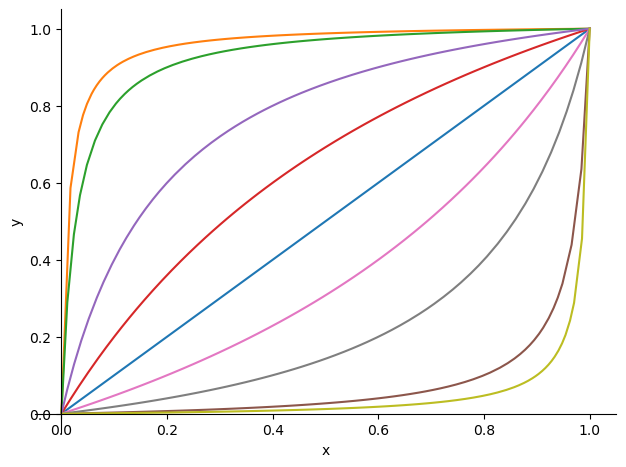
We can visualize contract curves with Cobb-Douglas utility functions
# Plot a range of αs and βs
params = [{α: 0.5, β: 0.5},
          {α: 0.1, β: 0.9},
          {α: 0.1, β: 0.8},
          {α: 0.8, β: 0.9},
          {α: 0.4, β: 0.8},
          {α: 0.8, β: 0.1},
          {α: 0.9, β: 0.8},
          {α: 0.8, β: 0.4},
          {α: 0.9, β: 0.1}]

p = plot(xlabel='x', ylabel='y', show=False)

for param in params:
    p_add = plot(sol.subs(param), (x, 0, 1),
                 show=False)
    p.append(p_add[0])
p.show()
Extra tasks:
Can you think of a way to draw the same graph using
numpy?How difficult will it be to write a
numpyimplementation?